
Xinyi Huang1, Raphael Horvath1, Andreas Hugi1
1) IRsweep AG, Laubisrütistr. 44, 8712 Stäfa, Switzerland
Introduction
Signal to noise is an important topic when discussing the performance of a spectrometer and a convenient way to describe this is through Allan deviation, which provides a way to quantify the noise present in a system as a function of integration time. In short, the Allan variance is calculated by dividing the measurement data into adjacent groups of equal length and taking the square of the difference between successive groups, divided by two. The Allan deviation is the square root of the Allan variance, just as the standard deviation is the square root of variance. This application note describes the result of applying an Allan deviation analysis to the output of the IRis-F1 and what this means for a measurement.
Results
The plots in Figure 1 show the noise behavior of the IRis-F1 with a laser module spanning approximately 1200 to 1290 cm-1. All measurements were done with an empty sample compartment and the absorbances are presented in log of base 10.
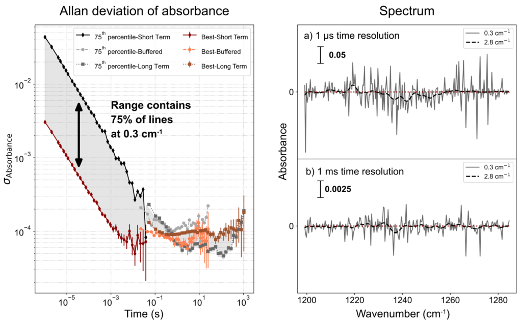
Allan plot of absorbance and spectra for different time resolutions and point spacing resolutions.
Allan deviation overview
The Allan deviation of two spectral points is shown on the left. It shows the standard deviation of a spectral line as a function of integration time. Since not all spectral points in a dual comb measurement are equal, two points are shown. The red and orange lines belong to the strongest heterodyne line, which has the lowest noise. The black and gray lines belong to the heterodyne line marking the 75th percentile. This means, 75% of the data points are better than this and lie in the range indicated.
The measurements span 1 µs to 1 hour. It’s currently not possible to do this in a single continuous measurement (watch this space for developments!), which is why three separate measurements were taken, represented by the lines Short Term, Buffered, and Long Term. The different acquisition modes are described elsewhere.
There can be a small jump in the vertical dimension when the acquisition mode is changed, which is due to different levels of throughput achieved. The Short Term measurement has a throughput of 100%, meaning all of the measurement time can be co-averaged. In contrast, the Long Term mode currently reaches a maximum throughput of ca. 10%, meaning that for every second measured, only 100 ms are integrated.
At short times, the Allan deviation decreases linearly with a slope of 0.5, which shows a dependence of noise on integration time (τ) of 1/√τ. At longer times, the dominant source of noise is due to long-term drifts and further averaging does not change the noise level. Different spectral lines take a different amount of time to converge to this same level. To improve further, see the section “Spectra overview”.
Spectra overview
The right side of the figure shows the spectral response of the IRis-F1 under several conditions. The top panel shows the noise at maximum time resolution of 1 µs, while the bottom panel shows the noise when integrated to 1 ms. From these plots, it’s easy to see how the noise is different across the spectral range and how it scales with integration time.
In each case, the black dashed line shows how the noise level improves with spectral integration. These figures were generated from a single acquisition. For even lower noise levels, acquisition-averaging can be used, which scales well for many hundreds of acquisitions. Otherwise, stronger spectral and/or time averaging is also possible. For example, with 1000 averages, τ of 500 µs, and 4 cm-1 spectral averaging, noise levels approaching 1 x 10⁻⁶ across a spectrum can be achieved.
Looking at all spectral lines
Looking at all lines of the Allan deviation can quickly become overwhelming. To improve visibility, Figure 2 shows all lines for this measurement ordered from worst to best in a heatmap. The axis Spectral Index therefore represents the wavenumber points, but ordered by noise level.
 Figure 2: Allan deviation for all spectral lines in the spectrum presented in order of deviation at the shortest integration time.
The break at 10-2 s once again represents a switch in acquisition modes (see above). Most of the spectral lines indicate outstanding noise for their integration times.
Related products
IRis-C
The IRis-C is the next generation instrument in IRsweep’s quantum cascade laser frequency comb spectrometer line. It uses the same dual-comb spectroscopy technology as IRsweep’s IRis-F1, offering microsecond time-resolution, high spectral resolution, and high optical brightness in the mid-infrared. With a substantial reduction in physical dimensions and price, it is easily adaptable to any type of application and fits even tighter budgets.
IRis-F1
The IRis-F1 spectrometer offers you an unmatched combination of speed, brightness and multi-color measurements. The quantum cascade laser frequency comb spectrometer is the first turn-key frequency comb spectroscopy system. As opposed to single-frequency operation, which necessitates tuning over your spectral range of interest, you will achieve a broad spectral coverage in a single-shot measurement.
IRis-core
The IRis-core is an ideal basis for the setup of such a system in the mid-IR range: It offers two overlapping free-running QCL-based frequency comb lasers in a single system. The system outputs already co-aligned beams and comes with a set of drive instructions with factory-characterized heterodyning conditions. The system comes complete with drive electronics and a control computer with a graphical user interface.